Overview

You’re probably not going to implement your own storage engine from scratch, but you do need to select a storage engine that is appropriate for your application.

Data Structures That Power Your Database

In order to efficiently find the value for a particular key in the database, we need a different data structure: an index.

This is an important trade-off in storage systems: well-chosen indexes speed up read queries, but every index slows down writes. For this reason, databases don’t usually index everything by default, but require you—the application developer or database administrator—to choose indexes manually, using your knowledge of the application’s typical query patterns.

Hash Indexes

Key-value stores are quite similar to the dictionary type that you can find in most programming languages, and which is usually implemented as a hash map (hash table).

Bitcask(the default storage engine in Riak) offers high-performance reads and writes, subject to the requirement that all the keys fit in the available RAM, since the hash map is kept completely in memory.

A storage engine like Bitcask is well suited to situations where the value for each key is updated frequently. For example, the key might be the URL of a cat video, and the value might be the number of times it has been played (incremented every time someone hits the play button). In this kind of workload, there are a lot of writes, but there are not too many distinct keys—you have a large number of writes per key, but it’s feasible to keep all keys in memory.

How do we avoid eventually running out of disk space? A good solution is to break the log into segments of a certain size by closing a segment file when it reaches a certain size, and making subsequent writes to a new segment file. We can then perform compaction on these segments. Compaction means throwing away duplicate keys in the log, and keeping only the most recent update for each key. Since compaction often makes segments much smaller (assuming that a key is overwritten several times on average within one segment), we can also merge several segments together at the same time as performing the compaction.

Important issue:

• File format
  • CSV is not the best format for a log. It’s faster and simpler to use a binary format that first encodes the length of a string in bytes, followed by the raw string (without need for escaping).
• Deleting records
  • If you want to delete a key and its associated value, you have to append a special deletion record to the data file (sometimes called a tombstone). When log segments are merged, the tombstone tells the merging process to discard any previous values for the deleted key.
• Crash recovery
  • If the database is restarted, the in-memory hash maps are lost. In principle, you can restore each segment’s hash map by reading the entire segment file from beginning to end and noting the offset of the most recent value for every key as you go along. However, that might take a long time if the segment files are large, which would make server restarts painful. Bitcask speeds up recovery by storing a snapshot of each segment’s hash map on disk, which can be loaded into memory more quickly.
• Partially written records
  • The database may crash at any time, including halfway through appending a record to the log. Bitcask files include checksums, allowing such corrupted parts of the log to be detected and ignored.
• Concurrency control
  • As writes are appended to the log in a strictly sequential order, a common implementation choice is to have only one writer thread. Data file segments are append-only and otherwise immutable, so they can be read concurrently by multiple threads.

An append-only log seems wasteful at first glance: why don’t you update the file in place, overwriting the old value with the new value? Reasons:

• Appending and segment merging are sequential write operations, which are generally much faster than random writes, especially on magnetic spinning-disk hard drives. To some extent sequential writes are also preferable on flash-based solid state drives (SSDs). We will discuss this issue further in “Comparing B-Trees and LSM-Trees”.
• Concurrency and crash recovery are much simpler if segment files are append-only or immutable. For example, you don’t have to worry about the case where a crash happened while a value was being overwritten, leaving you with a file containing part of the old and part of the new value spliced together.
• Merging old segments avoids the problem of data files getting fragmented over time.

Hash table index limitations:

• The hash table must fit in memory, so if you have a very large number of keys, you’re out of luck. In principle, you could maintain a hash map on disk, but unfortunately it is difficult to make an on-disk hash map perform well. It requires a lot of random access I/O, it is expensive to grow when it becomes full, and hash collisions require fiddly logic.
• Range queries are not efficient. For example, you cannot easily scan over all keys between kitty00000 and kitty99999—you’d have to look up each key individually in the hash maps.

SSTables and LSM-Trees

With Sorted String Table(SSTable), we require the sequence of key-value pairs is sorted by key. With this format, we cannot append new key-value pairs to the segment immediately, since writes can occur in any order; we will see shortly how to write SSTable segments using sequential I/O.

Advantages of SSTables over log segments:

• Merging segments is simple and efficient, even if the files are bigger than the available memory.
• In order to find a particular key in the file, you no longer need to keep an index of all the keys in memory.
• Since read requests need to scan over several key-value pairs in the requested range anyway, it is possible to group those records into a block and compress it before writing it to disk.

Constructing and maintaining SSTables

Maintaining a sorted structure on disk is possible (see “B-Trees”), but maintaining it in memory is much easier. There are plenty of well-known tree data structures that you can use, such as red-black trees or AVL trees. With these data structures, you can insert keys in any order and read them back in sorted order.

We can now make our storage engine work as follows:

• When a write comes in, add it to an in-memory balanced tree data structure (for example, a red-black tree). This in-memory tree is sometimes called a memtable.
• When the memtable gets bigger than some threshold—typically a few megabytes—write it out to disk as an SSTable file. This can be done efficiently because the tree already maintains the key-value pairs sorted by key. The new SSTable file becomes the most recent segment of the database. While the SSTable is being written out to disk, writes can continue to a new memtable instance.
• In order to serve a read request, first try to find the key in the memtable, then in the most recent on-disk segment, then in the next-older segment, etc.
• From time to time, run a merging and compaction process in the background to combine segment files and to discard overwritten or deleted values.

Problem: if the database crashes, the most recent writes (which are in the memtable but not yet written out to disk) are lost. In order to avoid that problem, we can keep a separate log on disk to which every write is immediately appended, just like in the previous section. That log is not in sorted order, but that doesn’t matter, because its only purpose is to restore the memtable after a crash. Every time the memtable is written out to an SSTable, the corresponding log can be discarded.

Making an LSM-Tree out of SSTables

Used in LevelDB and RocksDB, key-value storage engine libraries that are designed to be embedded into other applications. Among other things, LevelDB can be used in Riak as an alternative to Bitcask. Similar storage engines are used in Cassandra and HBase, both of which were inspired by Google’s Bigtable paper.

Log-Structured Merge-Tree(LSM-Tree) building on earlier work on log-structured filesystems. Storage engines that are based on this principle of merging and compacting sorted files are often called LSM storage engines.

B-Trees

B-trees keep key-value pairs sorted by key, which allows efficient key-value lookups and range queries. B-trees break the database down into fixed-size blocks or pages, traditionally 4 KB in size (sometimes bigger), and read or write one page at a time. This design corresponds more closely to the underlying hardware, as disks are also arranged in fixed-size blocks.

One page is designated as the root of the B-tree; whenever you want to look up a key in the index, you start here. The page contains several keys and references to child pages. Each child is responsible for a continuous range of keys, and the keys between the references indicate where the boundaries between those ranges lie.

The number of references to child pages in one page of the B-tree is called the branching factor. The branching factor depends on the amount of space required to store the page references and the range boundaries, but typically it is several hundred.

This algorithm ensures that the tree remains balanced: a B-tree with n keys always has a depth of O(log n). Most databases can fit into a B-tree that is three or four levels deep, so you don’t need to follow many page references to find the page you are looking for. (A four-level tree of 4 KB pages with a branching factor of 500 can store up to 256 TB.)

Making B-Trees Reliable

In order to make the database resilient to crashes, it is common for B-tree implementations to include an additional data structure on disk: a write-ahead log (WAL, also known as a redo log). This is an append-only file to which every B-tree modification must be written before it can be applied to the pages of the tree itself. When the database comes back up after a crash, this log is used to restore the B-tree back to a consistent state.

An additional complication of updating pages in place is that careful concurrency control is required if multiple threads are going to access the B-tree at the same time—otherwise a thread may see the tree in an inconsistent state. This is typically done by protecting the tree’s data structures with latches (lightweight locks). Log-structured approaches are simpler in this regard, because they do all the merging in the background without interfering with incoming queries and atomically swap old segments for new segments from time to time.

B-Tree optimization

• Instead of overwriting pages and maintaining a WAL for crash recovery, some databases (like LMDB) use a copy-on-write scheme. A modified page is written to a different location, and a new version of the parent pages in the tree is created, pointing at the new location. This approach is also useful for concurrency control, as we shall see in “Snapshot Isolation and Repeatable Read”.
• We can save space in pages by not storing the entire key, but abbreviating it. Especially in pages on the interior of the tree, keys only need to provide enough information to act as boundaries between key ranges. Packing more keys into a page allows the tree to have a higher branching factor, and thus fewer levels.iii
• In general, pages can be positioned anywhere on disk; there is nothing requiring pages with nearby key ranges to be nearby on disk. If a query needs to scan over a large part of the key range in sorted order, that page-by-page layout can be inefficient, because a disk seek may be required for every page that is read. Many B-tree implementations therefore try to lay out the tree so that leaf pages appear in sequential order on disk. However, it’s difficult to maintain that order as the tree grows. By contrast, since LSM-trees rewrite large segments of the storage in one go during merging, it’s easier for them to keep sequential keys close to each other on disk.
• Additional pointers have been added to the tree. For example, each leaf page may have references to its sibling pages to the left and right, which allows scanning keys in order without jumping back to parent pages.
• B-tree variants such as fractal trees borrow some log-structured ideas to reduce disk seeks (and they have nothing to do with fractals).

Comparing B-Trees and LSM-Trees

LSM-trees are typically faster for writes, whereas B-trees are thought to be faster for reads. Reads are typically slower on LSM-trees because they have to check several different data structures and SSTables at different stages of compaction.

Advantages of LSM-Trees

LSM-trees are typically able to sustain higher write throughput than B-trees, partly because they sometimes have lower write amplification (although this depends on the storage engine configuration and workload), and partly because they sequentially write compact SSTable files rather than having to overwrite several pages in the tree. This difference is particularly important on magnetic hard drives, where sequential writes are much faster than random writes.

LSM-trees can be compressed better, and thus often produce smaller files on disk than B-trees. B-tree storage engines leave some disk space unused due to fragmentation: when a page is split or when a row cannot fit into an existing page, some space in a page remains unused. Since LSM-trees are not page-oriented and periodically rewrite SSTables to remove fragmentation, they have lower storage overheads, especially when using leveled compaction.

On many SSDs, the firmware internally uses a log-structured algorithm to turn random writes into sequential writes on the underlying storage chips, so the impact of the storage engine’s write pattern is less pronounced. However, lower write amplification and reduced fragmentation are still advantageous on SSDs: representing data more compactly allows more read and write requests within the available I/O bandwidth.

Other Indexing Structure

It is also very common to have secondary indexes. A secondary index can easily be constructed from a key-value index. The main difference is that in a secondary index, the indexed values are not necessarily unique; that is, there might be many rows (documents, vertices) under the same index entry. This can be solved in two ways: either by making each value in the index a list of matching row identifiers (like a postings list in a full-text index) or by making each entry unique by appending a row identifier to it. Either way, both B-trees and log-structured indexes can be used as secondary indexes.

Storing values with the index

The key in an index is the thing that queries search for, but the value can be one of two things: it could be the actual row (document, vertex) in question, or it could be a reference to the row stored elsewhere. In the latter case, the place where rows are stored is known as a heap file, and it stores data in no particular order (it may be append-only, or it may keep track of deleted rows in order to overwrite them with new data later). The heap file approach is common because it avoids duplicating data when multiple secondary indexes are present: each index just references a location in the heap file, and the actual data is kept in one place.

In some situations, the extra hop from the index to the heap file is too much of a performance penalty for reads, so it can be desirable to store the indexed row directly within an index. This is known as a clustered index.

A compromise between a clustered index (storing all row data within the index) and a nonclustered index (storing only references to the data within the index) is known as a covering index or index with included columns, which stores some of a table’s columns within the index. This allows some queries to be answered by using the index alone (in which case, the index is said to cover the query)

Clustered and covering indexes can speed up reads, but they require additional storage and can add overhead on writes. Databases also need to go to additional effort to enforce transactional guarantees, because applications should not see inconsistencies due to the duplication.

Multi-Column indexes

The most common type of multi-column index is called a concatenated index, which simply combines several fields into one key by appending one column to another (the index definition specifies in which order the fields are concatenated).

Keeping Everything in memory

Compared to main memory, disks are awkward to deal with. With both magnetic disks and SSDs, data on disk needs to be laid out carefully if you want good performance on reads and writes. However, we tolerate this awkwardness because disks have two significant advantages: they are durable (their contents are not lost if the power is turned off), and they have a lower cost per gigabyte than RAM.

As RAM becomes cheaper, the cost-per-gigabyte argument is eroded. Many datasets are simply not that big, so it’s quite feasible to keep them entirely in memory, potentially distributed across several machines. This has led to the development of in-memory databases.

When an in-memory database is restarted, it needs to reload its state, either from disk or over the network from a replica (unless special hardware is used). Despite writing to disk, it’s still an in-memory database, because the disk is merely used as an append-only log for durability, and reads are served entirely from memory. Writing to disk also has operational advantages: files on disk can easily be backed up, inspected, and analyzed by external utilities.

In-memory databases is providing data models that are difficult to implement with disk-based indexes. For example, Redis offers a database-like interface to various data structures such as priority queues and sets. Because it keeps all data in memory, its implementation is comparatively simple.

Recent research indicates that In-memory database architecture could be extended to support datasets larger than the available memory, without bringing back the overheads of a disk-centric architecture. The so-called anti-caching approach works by evicting the least recently used data from memory to disk when there is not enough memory, and loading it back into memory when it is accessed again in the future. This is similar to what operating systems do with virtual memory and swap files, but the database can manage memory more efficiently than the OS, as it can work at the granularity of individual records rather than entire memory pages.

Data Warehousing

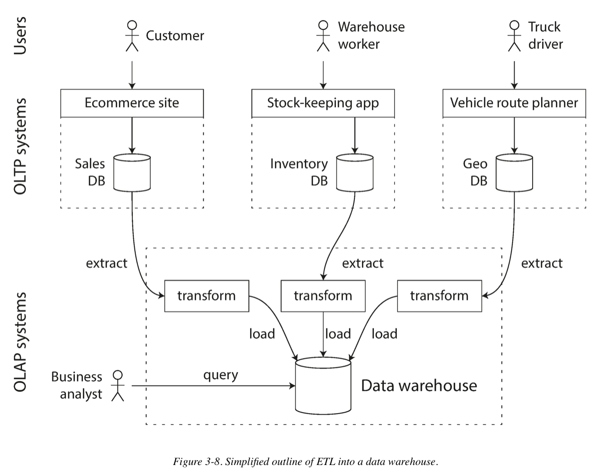
An enterprise may have dozens of different transaction processing systems: systems powering the customer-facing website, controlling point of sale (checkout) systems in physical stores, tracking inventory in warehouses, planning routes for vehicles, managing suppliers, administering employees, etc. Each of these systems is complex and needs a team of people to maintain it, so the systems end up operating mostly autonomously from each other.

These OLTP(online transaction processing) systems are usually expected to be highly available and to process transactions with low latency, since they are often critical to the operation of the business. Database administrators therefore closely guard their OLTP databases.

A data warehouse, by contrast, is a separate database that analysts can query to their hearts’ content, without affecting OLTP operations. The data warehouse contains a read-only copy of the data in all the various OLTP systems in the company. Data is extracted from OLTP databases (using either a periodic data dump or a continuous stream of updates), transformed into an analysis-friendly schema, cleaned up, and then loaded into the data warehouse. This process of getting data into the warehouse is known as Extract–Transform–Load (ETL).

A big advantage of using a separate data warehouse, rather than querying OLTP systems directly for analytics, is that the data warehouse can be optimized for analytic access patterns. It turns out that the indexing algorithms discussed in the first half of this chapter work well for OLTP, but are not very good at answering analytic queries. In the rest of this chapter we will look at storage engines that are optimized for analytics instead.

The divergence between OLTP Databases and Data Warehourse

The data model of a data warehouse is most commonly relational, because SQL is generally a good fit for analytic queries. There are many graphical data analysis tools that generate SQL queries, visualize the results, and allow analysts to explore the data (through operations such as drill-down and slicing and dicing).

Stars and Snowflakes: Schemas for Analytics

Star Schema(dimensional modeling): there is a center of schema is so called fact table. Each row of the fact table represents an event that occurred at a particular time.

Snowflake schema is dimensions are further broken down into subdimensions.

Snowflake schemas are more normalized than star schemas, but star schemas are often preferred because they are simpler for analysts to work with.

Column-Oriented Storage

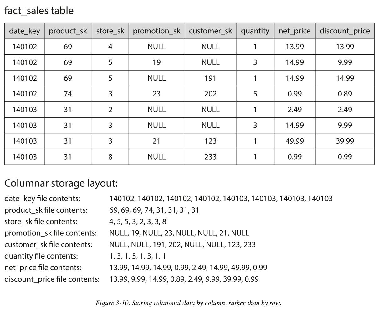
In most OLTP databases, storage is laid out in a row-oriented fashion: all the values from one row of a table are stored next to each other. Document databases are similar: an entire document is typically stored as one contiguous sequence of bytes.

The idea behind column-oriented storage is simple: don’t store all the values from one row together, but store all the values from each column together instead. If each column is stored in a separate file, a query only needs to read and parse those columns that are used in that query, which can save a lot of work.

Column Compression

Besides only loading those columns from disk that are required for a query, we can further reduce the demands on disk throughput by compressing data.

Memory bandwidth and vetorized processing

Besides reducing the volume of data that needs to be loaded from disk, column-oriented storage layouts are also good for making efficient use of CPU cycles. For example, the query engine can take a chunk of compressed column data that fits comfortably in the CPU’s L1 cache and iterate through it in a tight loop (that is, with no function calls). A CPU can execute such a loop much faster than code that requires a lot of function calls and conditions for each record that is processed. Column compression allows more rows from a column to fit in the same amount of L1 cache. Operators, such as the bitwise AND and OR described previously, can be designed to operate on such chunks of compressed column data directly. This technique is known as vectorized processing.

Writing to Column-Oriented Storage

These optimizations make sense in data warehouses, because most of the load consists of large read-only queries run by analysts. Column-oriented storage, compression, and sorting all help to make those read queries faster. However, they have the downside of making writes more difficult.

Aggregation: Data Cubes and Masterialized Views

Not every data warehouse is necessarily a column store: traditional row-oriented databases and a few other architectures are also used. However, columnar storage can be significantly faster for ad hoc analytical queries, so it is rapidly gaining popularity.

Materialized aggregates: data warehouse queries often involve an aggregate function, such as COUNT, SUM, AVG, MIN, or MAX in SQL. If the same aggregates are used by many different queries, it can be wasteful to crunch through the raw data every time. Why not cache some of the counts or sums that queries use most often?

One way of creating such a cache is a materialized view. In a relational data model, it is often defined like a standard (virtual) view: a table-like object whose contents are the results of some query. The difference is that a materialized view is an actual copy of the query results, written to disk, whereas a virtual view is just a shortcut for writing queries. When you read from a virtual view, the SQL engine expands it into the view’s underlying query on the fly and then processes the expanded query.

Summary

On a high level, we saw that storage engines fall into two broad categories: those optimized for transaction processing (OLTP), and those optimized for analytics (OLAP). There are big differences between the access patterns in those use cases:

• OLTP systems are typically user-facing, which means that they may see a huge volume of requests. In order to handle the load, applications usually only touch a small number of records in each query. The application requests records using some kind of key, and the storage engine uses an index to find the data for the requested key. Disk seek time is often the bottleneck here.
• Data warehouses and similar analytic systems are less well known, because they are primarily used by business analysts, not by end users. They handle a much lower volume of queries than OLTP systems, but each query is typically very demanding, requiring many millions of records to be scanned in a short time. Disk bandwidth (not seek time) is often the bottleneck here, and column-oriented storage is an increasingly popular solution for this kind of workload.

On the OLTP side, we saw storage engines from two main schools of thought:

• The log-structured school, which only permits appending to files and deleting obsolete files, but never updates a file that has been written. Bitcask, SSTables, LSM-trees, LevelDB, Cassandra, HBase, Lucene, and others belong to this group.
• The update-in-place school, which treats the disk as a set of fixed-size pages that can be overwritten. B-trees are the biggest example of this philosophy, being used in all major relational databases and also many nonrelational ones.

Log-structured storage engines are a comparatively recent development. Their key idea is that they systematically turn random-access writes into sequential writes on disk, which enables higher write throughput due to the performance characteristics of hard drives and SSDs.

Reference

https://www.amazon.com/Designing-Data-Intensive-Applications-Reliable-Maintainable/dp/1449373321