Definition

A decision tree is a decision support tool that uses a tree-like model of decisions and their possible consequences, including chance event outcomes, resource costs, and utility. It is one way to display an algorithm that only contains conditional control statements.

For decision tree for classification problems is a special form of binary tree, which is used as a classifier. There are two types of nodes in decision tree:

• leaf node: same as the ones in binary tree, i.e. the node that does not have any child node.
• decision node: the non-leaf node.

The decision node’s condition that control next child node:

• For numerical attributes, the condition takes the form of less-or-equal-than comparison, i.e. “${\text{object.attribute} \le C}$”. For example, ${\text{object.height} \le 1.7}$object.
• For categorical attributes, the condition is expressed as membership to a list of categorical values, i.e. ${\text{object.attribute} \in {C_1, C_2, C_3 …} }$. For example, ${\text{object.color} \in { \text{red, green, yellow} }}$.

How to build decision tree for classification problem

The algorithm to construct a decision tree follows the approach of divide-and-conquer, i.e. we recursivelly splitting the input samples into two subgroups with decision node, until we no longer need to split them. At the end, each of the samples is assigned to a leaf node, and we label the leaf node with the category of the majority samples within the leaf node.

We can recursively construct the tree:

• base cases: If the samples are of the same labels, then we do not need to further split the samples. This is the fundamental base case. One can define more base cases in order to regulate the complexity of the final tree.
• recurrence relation: We find the most distinguishable feature of the samples and also the best value to split on, in order to obtain two subgroups of samples. We then construct subtrees out of the split subgroups. The criterion to split the samples is twofold:
  • 1). we should reduce the samples into smaller scales in a fast manner, so that we could reduce the occurrence of recursion, i.e. reduce the cost of the algorithm.
  • 2). we should also make sure the split subgroups are more uniform so that it becomes easier to classify the samples.
• stop conditions
  • All the examples that fall into the current node belong to the same category, i.e. no further classification is needed.
  • The tree reaches its predefined max_depth
  • The number of examples that fall into the current node is less than the predefined minimal_number_of_examples.

Pseudo Code

TreeNode build_decision_tree([samples]) {
      
  // base cases:
      - the target attributes of the samples are uniform 
      - the current depth of tree exceeds the max_tree_depth
      - the number of samples is less than the minimal_node_size 

  // 1). we create a leaf node and return.
  if (any of the above cases holds) {
    leaf_node = create_leaf_node([samples]);
    return leaf_node;
  }
      
  // 2). find the best attribute to split on, (also the best value to split)
  feature_to_split, split_value = find_best_split([samples]);

  // 3). split the samples list into two sublists
  left_samples, right_samples = split([samples], feature_to_split, split_value);

  // 4). create a decision node.
  new_node = create_node(feature_to_split, split_value);

  // 5). for each sublist, recursively call the function to create the subtrees.
  new_node.left = build_decision_tree(left_samples);
  new_node.right = build_decision_tree(right_samples);

  // 6). return the newly-created node
  return new_node;
}

How to choose split criterion

Split purpose:

• The splitting reduces the problem into smaller ones, which eventually leads to the termination of the recursion process.
• The splitting criterion, i.e. the feature to split on and the value to split with, serves as the branching condition in the decision node.
• The splitted subgroups would be used as the input samples to further construct the left and right subtrees.

We should split the data which are more distinguishable. In order to find the best split:

• Which feature to split on?
• Which value of the chosen feature to split with?
• How can we evaluate the quality of the splits ?

Gini impurity - measure disorder on a group of values

Gini impurity can be applied to evaluate the quality of the splits. It is ultimately a metric that is intended to measure the impurity for a group of values, which is on the contrary of uniformity where all values are identical.

In the context of Decision Tree, the metric of gini impurity is used to evaluate the quality of a split, where we split a list of samples into two subgroups.

The more uniform for the samples in each group, the easier one can make a decision on how to classify a sample, i.e. the lower the gini impurity for a group, the easier we can assign the right label for the samples in the group.

Given a list of samples ${X}$ with ${n}$ unique values, we could obtain the Gini impurity of the group with the following formula:

we can also expand the above formula and rewrite it as follows:

where ${P(x_i)}$ is the probability of finding a sample with the value ${x_i}$ in a random sampling. The number of samples is greater and/or equal than $n$, where one can have multiple samples of the same value.

Example:

We have a group of 4 samples as [versicolor, setosa, setosa, setosa]. If we randomly select two samples from the group with replacement, then the probability that the two samples are of different values would be ${1 - \frac{1}{4} \cdot \frac{1}{4} - \frac{3}{4} \cdot \frac{3}{4} = \frac{3}{8} }$.

Gini Gain

The reduction of the gini impurity is also called “gini gain”. The quality of the split is measured by gini gain. The higher the gini gain, the better the split.

For a group ${L}$, we divide the group into two subgroups ${L_1, L_2}$, the gini gain of this split is defined as following:

The overall Gini impurity of split subgroups ${L_1, L_2}$, is the sum of Gini impurity for each subgroup weighted by its proportion with regards to the original group.

Example:

Apply the Gini gain to measure the quality of two splitting candidates for the group ${L}$ = [versicolor, setosa, setosa, setosa]:

• Candidate 1): ${L_1}$ = [versicolor, setosa], ${L_2}$ = [setosa, setosa].

• Candidate 2): ${L_1}$ = [versicolor], ${L_2}$ = [setosa, setosa, setosa].

Entropy - measure disorder on a group of values

Entropy can be defined as the unpredictability of the state. The more probable a state is, the less entropy that it has, i.e. the less information this state contains.

For a variable that has multiple states, its entropy is defined as the average of information content that each state contains.

For a discrete random variable $X$ with the possible values of ${ {x_1, …, x_n} }$, Shannon defined the entropy of $X$ as $H(X)$, as follows:

where $\mathbb{E}$ is the average function, $I(X)$ is the information content for each state of $X$.

Literally, we can interpret the entropy for the random ${X}$ is the average amount of information that it contains.

The above formula can be further expanded as follows:

where $P(x_i)$ is the probability for each state of $X$, and $I(x_i) = - {\log_{2} \mathrm{P}(x_i)}$.

The more likely a state $x_i$ (i.e. the bigger ${P(x_i)}$, the less information it contains (i.e. the smaller ${I(x_i)}$.

Example:

Given a group of values ${1, 1, 2, 2}$, we first calculate the probability for each unique vaue as: $P(1) = \frac{2}{4} = \frac{1}{2}$, $P(2) = \frac{2}{4} = \frac{1}{2}$.

Then, we can further obtain the entropy as: $- \frac{1}{2} \log_{2}{(\frac{1}{2})} - \frac{1}{2} \log_{2}{(\frac{1}{2})} = 1$

Information Gain

Entropy is a measure of disorder. The higher the entropy, the more disordered a group.

On the other hand, we can say that the more disorder a group is, the more entropy it has, i.e the more information it contains.

The entropy reduction is also known as information gain.

For a group ${L}$, we split it into two subgroups ${L_1, L_2}$, the information gain of the split is defined as follows:

The overall entropy of the split subgroups ${L_1, L_2}$, is the sum of the entropy for each subgroup weighted by its proportion with regards to the original group.

Example:

Apply the information gain to measure the quality of two splitting candidates for the group ${L}$ = [versicolor, setosa, setosa, setosa].

First of all, based on the formula of entropy, let us calculate the entropy of the group ${L}$ as follows:

• Candidate 1): ${L_1}$ = [versicolor, setosa], ${L_2}$ = [setosa, setosa].

• Candidate 2): ${L_1}$ = [versicolor], ${L_2}$ = [setosa, setosa, setosa].

Entropy VS. Gini Impurity

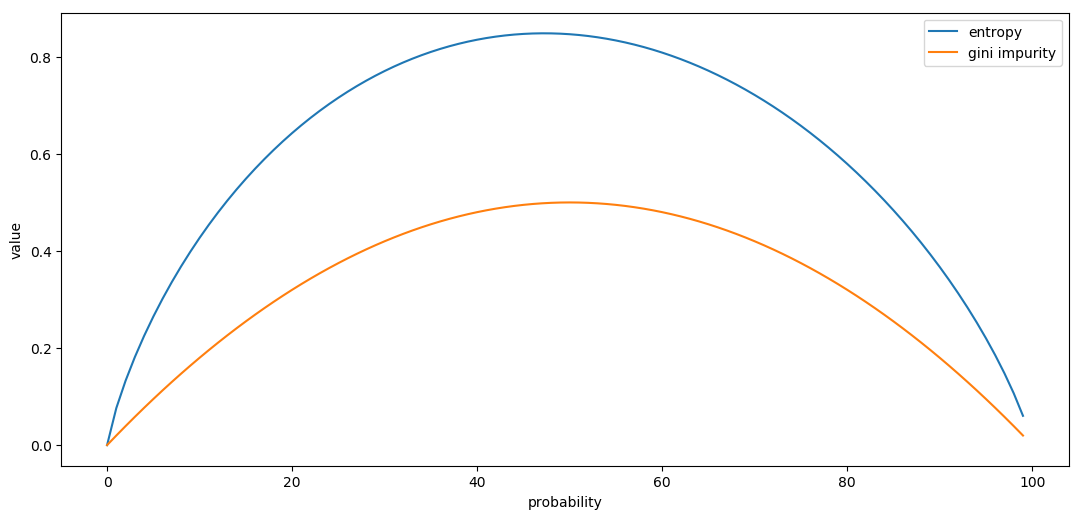
The X axis represents the probability $P$ for one of the two values in the group. Accordingly, the probability of the other value would be $(1-P)$. And the Y axis represents the entropy / Gini impurity of the group, given the probabilities of two values respectively.

• they are both of bell shape, e.g. both metrics reach their maximum when the two values are equally likely to appear (P = 50\%P=50%), in which case we can say the group is the most chaotic, since we have the least certainty to determine the value of a random sample.
• entropy metric has a larger scale than the Gini impurity, i.e. at each point of probability, the entropy value of the group is bigger than its Gini impurity.
• entropy metric provides a sharper contrast between a chaotic group and a less chaotic one, as we can see that the curve of entropy is steeper than the Gini impurity one.
• both metrics are capable to measure the quality of splits. Yet, entropy is a bit more expensive to calculate, in terms of computing.

To summarize, in general, there is no fundamental difference between entropy and Gini impurity. They are both suitable to measure the quality of split during the process of decision tree construction.

Precision VS. Recall - measure performance of classification model

• Precision: “How many selected items are relevant?”
• Recall: “How many relevant items are selected?”

There are 4 cases:

• True Positive (${T_p}$): For a picture, if the predicted class is positive (i.e. cat) and the actual class of the picture happens to be positive as well, we then call this case as True Positive.
• True Negative (${T_n}$): For a picture, if the predicated class is negative (i.e. non-cat) and the actual class happens to be negative as well, we then call this case as True Negative.
• False Positive (${F_p}$): For a picture, if the predicted class is positive (i.e. cat), but the actual class of the picture is negative (i.e. non-cat), we then call this case as False Positive.
• False Negative (${F_n}$): For a picture, if the predicated class is negative (i.e. non-cat), but the actual class of the picture is positive (i.e. cat), we then call this case as False Negative.

Define the metrics of Precision and Recall:

• Precision (${P}$) is defined as the ratio between the number of true positives (${T_p}$) and the number of all positive prediction (${T_p + F_p}$), i.e. the number of true positives plus the number of false positives. ${P = \frac{T_p}{T_p + F_p} }$
  • Precision metric is certainty when classifier claims the sample as positive
• Recall (${R}$) is defined as the ratio between the number of true positives (${T_p}$) and the number of all positive samples (${T_p + F_n}$), i.e. the number of true positives plus the number of false negatives. ${R = \frac{T_p}{T_p + F_n}}$
  • Recall metrics is percentage of how many of those actual positive cases are identified by the classifier.

Accuracy - measure performance of classification model

The accuracy (${A}$) is defined as the proportion of true results (including true positives (${T_p}$) and true negatives (${T_n}$) with regards to all the predictions (${T_p + T_n + F_p + F_n}$).

Comparing to Precision-Recall, the accuracy seems to be a more balanced metric, since it takes into account both True Positives and True Negatives.

However, it turns out that accuracy is actually a misleading metric, especially for the imbalanced datasets. For example, for a data set with 5 spam emails (i.e. positive samples) and 95 normal emails (i.e. negative samples), a naive spam classifier that simply predicts all samples as negatives (non-spam) would score a high accuracy of 95%. While measuring with Precision-Recall metrics, the spam classifier has zero precision and recall, which tells more accurately the actual predicting power of the classifier.

As a result, in practice people prefer the Precision-Recall metric over the accuracy as the measurement to benchmark their classifiers.

Reference

• https://en.wikipedia.org/wiki/Decision_tree